Positioning Sankey elements

Using `position_sankey`

Positioning elements in a Sankey / alluvial diagram is controlled with the position_sankey() function. It can be used to set spacing between nodes (see Spacing); Apply vertical alignment (see Alignment); Introduce a split within a stage (see Splitting nodes); Alter the stacking order (see Stacking order); Nudge positions (see Nudging).

In order to illustrate the positioning options, ?ecosystem_services data is used which comes packaged with ggsankeyfier.

library(ggplot2)
library(ggsankeyfier)
theme_set(theme_light())
data("ecosystem_services")

Please check vignette("data_management") if you wish to understand how this data was pre-processed.

Spacing

There are three important parameters when setting up the spacing in a Sankey diagram:

width: which specifies the combined width of a node in a specific stage. When the nodes are split up, each half will have a width of width / 2.
h_space: is the horizontal space (specified in native units) between split nodes (measured from the center of each half).
v_space: is the minimal vertical space between nodes measured in native units. Depending on the alignment of nodes this spacing might be stretched.

This is illustrated in the following example:

pos <- position_sankey(split_nodes = TRUE, align = "top",
                       width = 0.2, v_space = 0.15, h_space = 0.25)
serv_plot <-
  ggplot(ecosystem_services_pivot1,
         aes(x = stage, y = RCSES, group = node, connector = connector,
             edge_id = edge_id)) +
  geom_sankeyedge(position = pos) +
  geom_sankeynode(position = pos)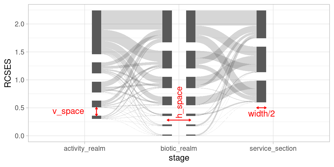

Alignment

Vertical alignment can be controlled with the align argument. Alignment is explained with the plot shown below. There, two red horizontal dashed guide lines are used to snap the different alignment options.

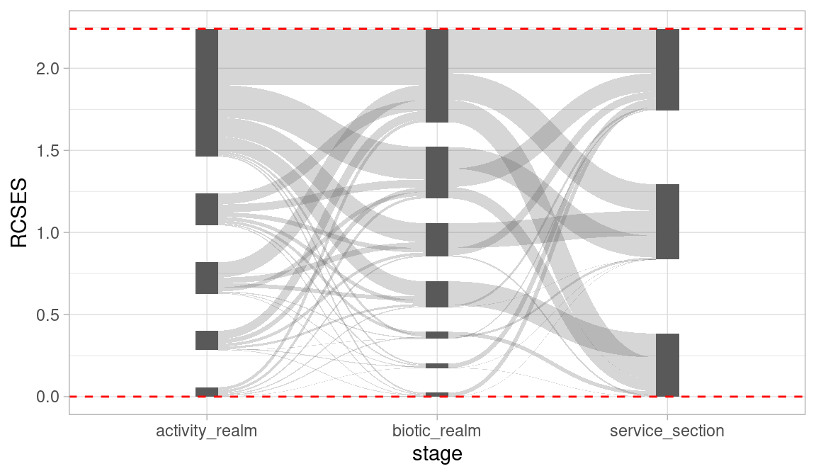
When align = 'justified', nodes in each stage are spread (by varying the vertical space) such that they line up with the top and bottom guide lines. The minimum space between nodes is controlled with v_space.

When align = 'top' or 'bottom', nodes are aligned with the top or bottom guide line respectively, where the v_space will be constant.

When align = 'center', nodes are centered around the middle between the top and bottom guide lines, where v_space will be constant.

When you are working with split_nodes = TRUE, alignment will be a more tedious job.

Splitting nodes

When split_nodes = TRUE, a vertical split is introduced for each node in a stage. This split can be useful when you wish to emphasise transitions between stages. It can also be used to show an imbalance when edges flowing from and to nodes are not equal. This imbalance is shown in the example below, by selecting a subset of edges. Note that a split is introduced automatically when edges flowing from and to a node are not equal.

es_sub <- ecosystem_services_pivot2 |> subset(RCSES > quantile(RCSES, 0.9))
ggplot(es_sub,
       aes(x = stage, y = RCSES, group = node, connector = connector, edge_id = edge_id)) +
  geom_sankeyedge(aes(fill = service_section)) +
  geom_sankeynode()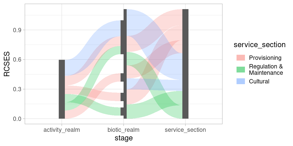

Stacking order

Another aspect you might want to control in a Sankey diagram is the stacking order of the nodes and edges. When order = "as_is", the nodes will be stacked in the order of their levels (or order of appearance), the edges will be arranged in the order of edge_id (or their order of appearance). Other options are order = "ascending" and order = "descending", both of which are based on the y aesthetic.

In order to demonstrate the stacking order we reduce the number of records from the example data (i.e., only select the higher risk chains from the data). This will produce a less cluttered Sankey diagram.

es_sub <-
  ecosystem_services |>
  subset(RCSES > quantile(RCSES, 0.99)) |>
  pivot_stages_longer(c("activity_realm", "biotic_realm", "service_section"),
                      "RCSES", "service_section")

p <- ggplot(es_sub,
       aes(x = stage, y = RCSES, group = node, connector = connector,
           edge_id = edge_id))

This will plot the nodes and edges in ascending stacking order (largest at the top):

pos <- position_sankey(v_space = "auto", order = "ascending")
p + geom_sankeyedge(aes(fill = service_section), position = pos) +
  geom_sankeynode(position = pos)

This will plot the nodes and edges in desacending stacking order (largest at the bottom):

pos <- position_sankey(v_space = "auto", order = "descending")
p + geom_sankeyedge(aes(fill = service_section), position = pos) +
  geom_sankeynode(position = pos)

Nudging

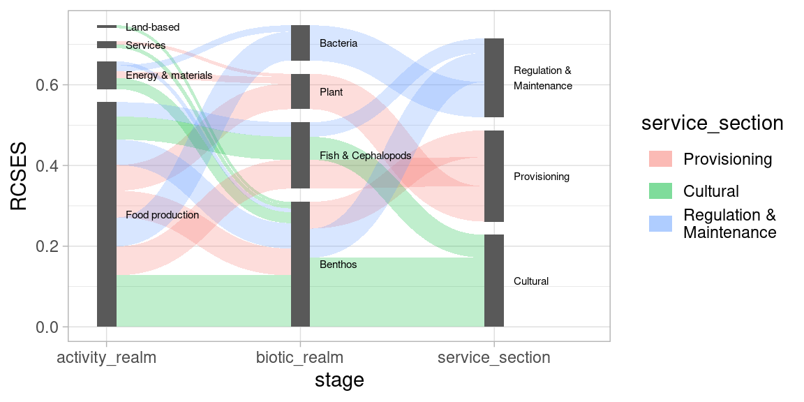
The function position_sankey() can also be used to position text labels. Let’s use it to add labels to the nodes. Note that we are using a simple ggplot2::geom_text() layer, where we provide "sankeynode" as stat function and the pos object for positioning the labels.

pos <- position_sankey(v_space = "auto", order = "descending")
p + geom_sankeyedge(aes(fill = service_section), position = pos) +
  geom_sankeynode(position = pos) +
  geom_text(aes(label = node), stat = "sankeynode", position = pos, cex = 2)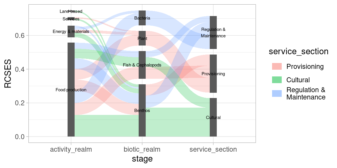

Let’s say you want to place the text labels next to the nodes. In that case you need to nudge the calculated into the desired position. We also need to adjust the justification of the text labels and expand the x scales.