Position nodes and edges in a Sankey diagram

Calculates the x and y positions of elements (nodes and edges) in a Sankey diagram.

Usage

PositionSankey

position_sankey(
  width = "auto",
  align = c("bottom", "top", "center", "justify"),
  order = c("ascending", "descending", "as_is"),
  h_space = "auto",
  v_space = 0,
  nudge_x = 0,
  nudge_y = 0,
  split_nodes = FALSE,
  split_tol = 0.001,
  direction = c("forward", "backward"),
  ...
)

Format

An object of class PositionSankey (inherits from Position, ggproto, gg) of length 13.

Arguments

width

Width of the node (numeric). When split_nodes is set to TRUE each part of the split node will have half this width. Use "auto" to automatically determine a suitable width.

align

A character that indicates how the nodes across the stages are aligned. It can be any of "top", "bottom", "center" or "justify".

order

A character indicating the method to be used for the order of stacking nodes and edges in a plot. Should be one of: ascending (default), sorts nodes and edges from large to small (largest on top); descending sorts nodes and edges from small to large (smallest on top); as_is will leave the order of nodes and edges as they are in data.

h_space

Horizontal space between split nodes (numeric). This argument is ignored when split_nodes == FALSE. Use "auto" to automatically position split nodes.

v_space

Vertical space between nodes (numeric). When set to zero (0), the Sankey diagram becomes an alluvial plot. Use "auto" to automatically determine a suitable vertical space.

nudge_x, nudge_y

Horizontal and vertical adjustment to nudge items by. Can be useful for offsetting labels.

split_nodes

A logical value indicating whether the source and destination nodes should be depicted as separate boxes.

split_tol

When the relative node size (resulting source and destination edges) differs more than this fraction, the node will be displayed as two separate bars.

direction

One of "forward" (default) or "backward". When set to "backward" the direction of the edges will be inverted. In most cases this parameter won't affect the plot. It can be helpful when you want to decorate the end of an edge (instead of the start; see examples).

...

Arguments passed on to ggplot2::ggproto().

Value

Returns a ggplot2::Position class object.

Details

Based on the stat_* function applied to the parent's (stat_sankeynode(), stat_sankeyedge) object either node or edge positions are calculated respectively. These positions can be used to add additional layers (e.g., text or labels) to the plot.

Author

Pepijn de Vries

Examples

library(ggplot2)
data("ecosystem_services")

pos  <- position_sankey(v_space = "auto", order = "ascending")
pos2 <- position_sankey(v_space = "auto", order = "ascending", direction = "backward")

## Let's subset the data, to make the plot less cluttered:
es_subset <- pivot_stages_longer(
  subset(ecosystem_services, RCSES > 0.01),
  c("activity_realm", "biotic_realm", "service_section"),
  "RCSES",
  "service_section"
)


plot <-
  ggplot(es_subset, aes(x = stage, y = RCSES, group = node,
                                    connector = connector, edge_id = edge_id,
                                    fill = node)) +
  geom_sankeynode(position = pos) +
  geom_sankeyedge(position = pos, aes(fill = service_section))

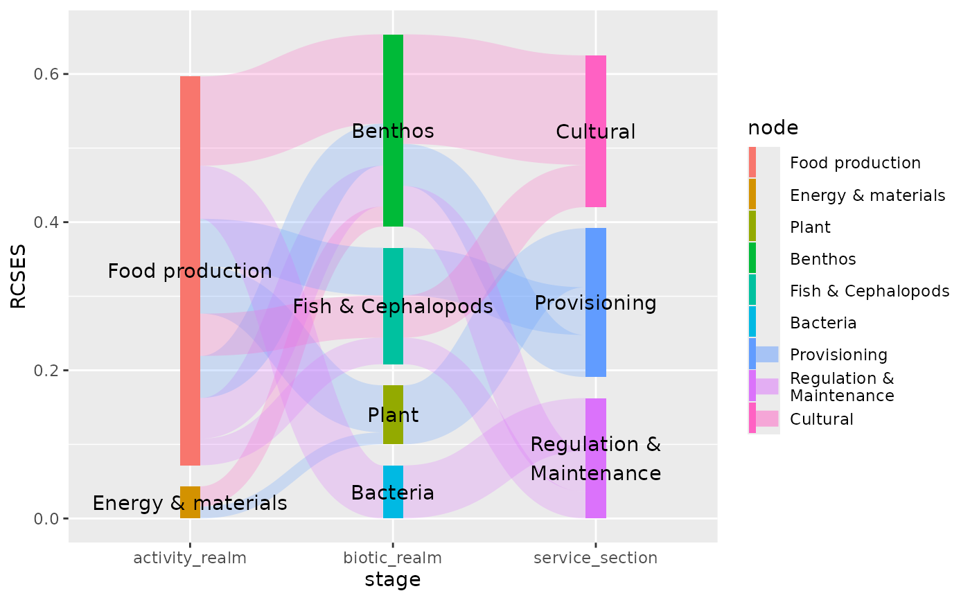
# position labels at nodes
plot + geom_text(aes(label = node), stat = "sankeynode", position = pos)

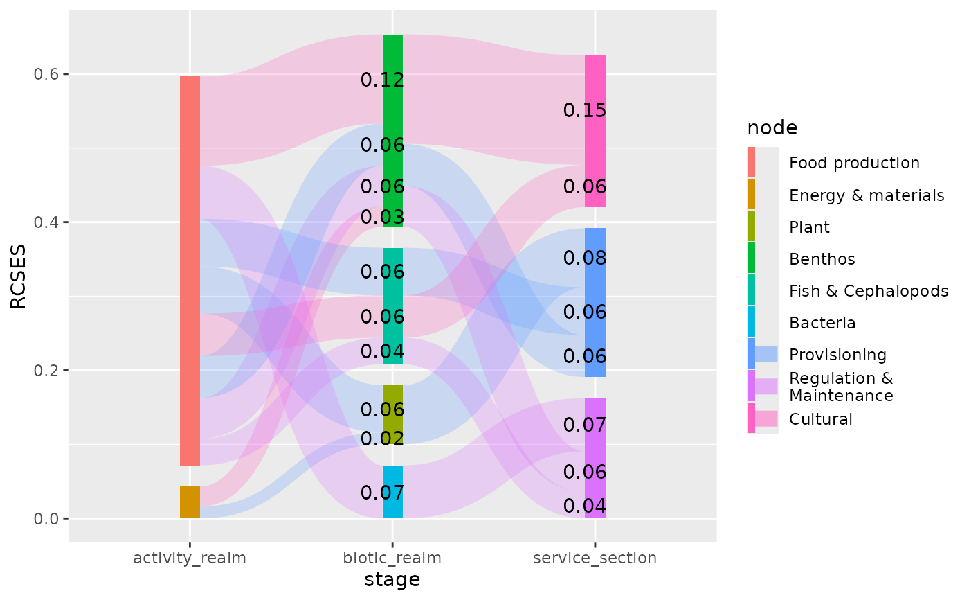
# position labels at the start of edges
plot + geom_text(aes(label = sprintf("%0.2f", RCSES)), stat = "sankeyedge", position = pos)

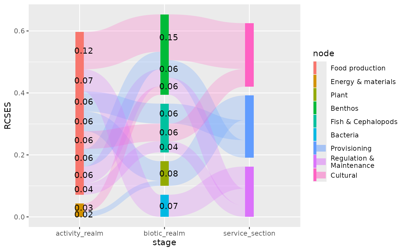# position labels at the end of edges
plot + geom_text(aes(label = sprintf("%0.2f", RCSES)), stat = "sankeyedge", position = pos2)