This vignette presents some vital aspects of decorating your plot with solar cylce information
## load required namespaces for this vignette
library(ggplot2)
library(gghourglass)
With annotate_daylight() you can add ribbons to your
plot reflecting the solar cycle. By default, it marks the time between
sunset and sunrise:
## get example data
data(bats)

## subset example date to the year 2018
bats_sub <- subset(bats, format(RECDATETIME, "%Y") == "2019")

## retrieve monitoring location
lon <- attr(bats, "monitoring")$longitude[1]
lat <- attr(bats, "monitoring")$latitude[1]

## plot the data
p <- ggplot(bats_sub, aes(x = RECDATETIME)) +

    ## add hourglass geometry to plot
    geom_hourglass() +

    ## add informative labels
    labs(x = "Date", y = "Time of day")

## decorate the plot with night time ribbon
p + annotate_daylight(lon, lat, c("sunset", "sunrise"), fill = "darkblue")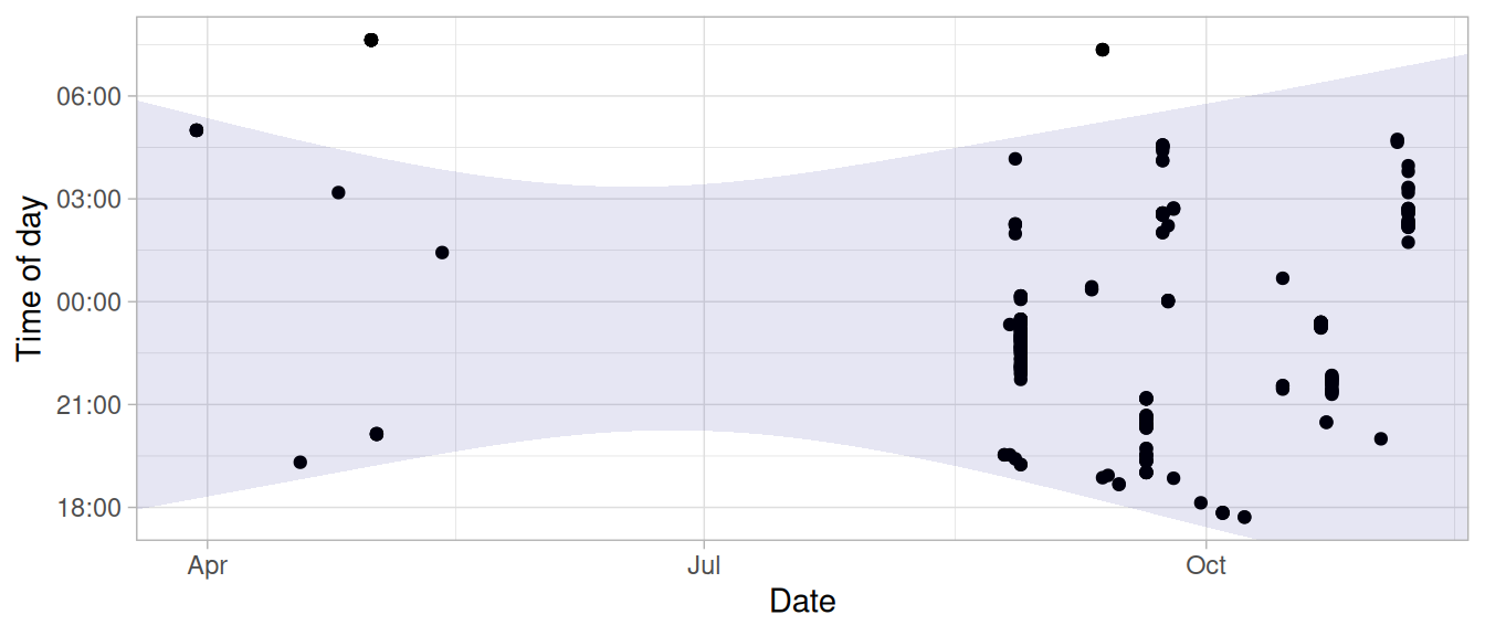
The order in which you include the solar events matter. In the example above, the time between sunset and sunrise (i.e., night time) is marked with a dark blue ribbon. But if you reverse the order, it will mark the day time:
p + annotate_daylight(lon, lat, c("sunrise", "sunset"), fill = "orange")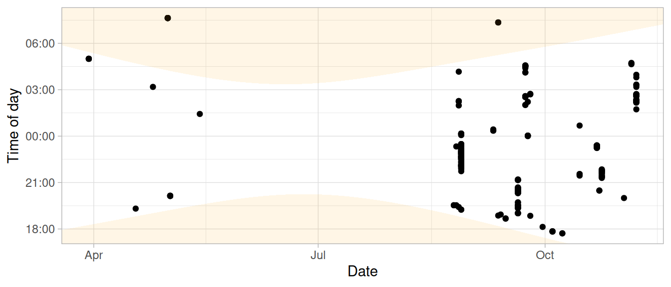
Moreover, you are not bound to only sunrise and sunset. You can pick any of the events supported by the suncalc package:
- solarNoon
- nadir
- sunrise
- sunset
- sunriseEnd
- sunsetStart
- dawn
- dusk
- nauticalDawn
- nauticalDusk
- nightEnd
- night
- goldenHourEnd
- goldenHour