Tidy csquares

The Csquares family

csquares objects can inherit properties from different parents as illustrated in vignette("csquares-objects"). When a csquares object inherits from the class data.frame(), you can apply many tidyverse operations while preserving the csquares properties of the object. When you create a csquares object from a character(), you cannot use tidyverse operations as it doesn’t inherit the data.frame() class. You can check which ancestors your object has by calling class() as shown in the example below.

## Required libraries
library(csquares)
library(dplyr)
library(sf)
library(ggplot2)

## create a simple csquares object:
char_csq <- as_csquares(c("1000", "3000"))

## This simple objects has "character" as parent class.
## So tidyverse is out of the question here.
class(char_csq)
#> [1] "csquares"   "character"  "vctrs_vctr"

So let’s start by creating a csquares object that does inherit from the data.frame() class. It will be used in examples shown in this vignette.

## create a csquares object with geometries:
orca_csq  <- orca |> as_csquares(csquares = "csquares")

## It inherits the class data.frame.
class(orca_csq)
#> [1] "csquares"   "data.frame"

Tidyverse operations

All tidyverse (and base) methods implemented in the Csquares package end with the suffix .csquares. You should never call these functions directly as this will likely produce errors. Instead, load the packages that implement the generic method (e.g., dplyr for mutate() and summarise(); tidyr for pivot_wider(); sf for st_as_sf() etc.). Then call the method without the .csquares suffix as shown in the examples below. As you call the method on csquares objects, the correct implementation of the generic method will be dispatched automatically.

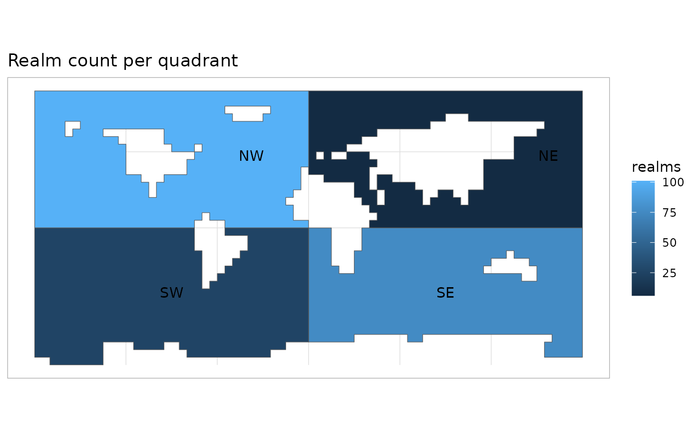
The example below shows how you can mutate a column in a csquares object, then group by a specific column and summarise it. The csquares properties are grouped automatically. If the csquares object inherits spatial features, the geometries are recalculated after summarising.

orca_sum <-
  orca_csq |>
## Add geometries to the object
  st_as_sf() |>
  ## use `mutate` to create a column that contains the csquares' quadrant
  mutate(quadrant = case_match(substr(csquares |> as.character(), 1L, 1L),
                               "1" ~ "NE", "3" ~ "SE", "5" ~ "SW", "7" ~ "NW")) |>
  ## grouping by the column with logical values and summarising
  ## will reduce the number of rows to 4 (one for each quadrant)
  group_by(quadrant) |>
  summarise(realms = sum(orcinus_orca), .groups = "keep")

## Note that csquares are automatically concatted and
## geometries recalculated
ggplot(orca_sum) +
  geom_sf(aes(fill = realms)) +
  geom_sf_text(aes(label = quadrant)) +
  coord_sf() +
  labs(title = "Realm count per quadrant", x = NULL, y = NULL)

Printing the summarised object shows that there are only two rows left. One for each value in the grouped column.

orca_sum
#> Simple feature collection with 4 features and 3 fields
#> Geometry type: POLYGON
#> Dimension:     XY
#> Bounding box:  xmin: -180 ymin: -90 xmax: 180 ymax: 90
#> Geodetic CRS:  WGS 84
#> # A tibble: 4 × 4
#> # Groups:   quadrant [4]
#>   quadrant realms csquares                                                  geom
#> * <chr>     <int> <csquares>                                       <POLYGON [°]>
#> 1 NE            6 1004:1|1004:2|1004:4|1005:1|1005:2|… ((10 35, 5 35, 0 35, 0 4…
#> 2 NW          101 7000:1|7000:2|7001:1|7001:2|7001:3|… ((-180 10, -180 15, -180…
#> 3 SE           76 3000:1|3000:2|3000:3|3000:4|3001:1|… ((0 -55, 0 -50, 0 -45, 0…
#> 4 SW           26 5000:1|5000:2|5000:3|5000:4|5001:1|… ((-180 -85, -180 -80, -1…

Join

Joining csquares objects is pretty straightforward and is only allowed on objects that inherit from the data.frame class. An exception are csquares objects that inherit from the stars class (stars::st_as_stars()). On those objects you are allowed to perform left joins, all other joins are impossible. See also ?join.

Below you see how you can simply join a data.frame to a csquares object by the csquares code.

df <- data.frame(foo = "bar", csquares = "3603:3")

left_join(orca_csq, df, by = "csquares") |> print(max = 30)
#>         csquares orcinus_orca  foo
#> 1  S60 E 30 (5°)        FALSE  bar
#> 2  S60 W 40 (5°)        FALSE <NA>
#> 3  N10 W 90 (5°)         TRUE <NA>
#> 4  N 0 W 40 (5°)        FALSE <NA>
#> 5  S10 W 70 (5°)         TRUE <NA>
#> 6  N 0 W100 (5°)         TRUE <NA>
#> 7  N40 E 30 (5°)        FALSE <NA>
#> 8  N 0 W100 (5°)         TRUE <NA>
#> 9  S 0 W 10 (5°)        FALSE <NA>
#> 10 S40 E130 (5°)         TRUE <NA>
#>  [ reached 'max' / getOption("max.print") -- omitted 2048 rows ]
right_join(orca_csq, df, by = "csquares")
#>        csquares orcinus_orca foo
#> 1 S60 E 30 (5°)        FALSE bar

You are also allowed to join a csquares object to another csquares by another column that does not represent the csquares codes:

csq <- data.frame(orcinus_orca = FALSE, csquares = "3603:3") |>
  as_csquares(csquares = "csquares")

left_join(orca_csq, csq, by = "orcinus_orca") |> print(max = 30)
#>       csquares.x orcinus_orca    csquares.y
#> 1  S60 E 30 (5°)        FALSE S60 E 30 (5°)
#> 2  S60 W 40 (5°)        FALSE S60 E 30 (5°)
#> 3  N10 W 90 (5°)         TRUE         empty
#> 4  N 0 W 40 (5°)        FALSE S60 E 30 (5°)
#> 5  S10 W 70 (5°)         TRUE         empty
#> 6  N 0 W100 (5°)         TRUE         empty
#> 7  N40 E 30 (5°)        FALSE S60 E 30 (5°)
#> 8  N 0 W100 (5°)         TRUE         empty
#> 9  S 0 W 10 (5°)        FALSE S60 E 30 (5°)
#> 10 S40 E130 (5°)         TRUE         empty
#>  [ reached 'max' / getOption("max.print") -- omitted 2048 rows ]

Note that the resulting csquares object has two columns with csquares codes. Only the column from the left-hand table in the join is used for further operations. However, you should wonder if this join is meaningful when mismatching csquares codes are the result.

The Csquares family

Tidyverse operations

Join

Further reading