Wildcards • csquares

What are wildcards?

Wildcards are special characters that represent any valid alternative character. In the context of c-squares, wildcards can be used to compactly notate a range of raster cells. Let’s say you have the following string of four c-squares defined:

library(csquares)

csq <- as_csquares("1000:1|1000:2|1000:3|1000:4")

print(csq)
#>  csquares [1:1]   4 squares

These are four squares of 5° by 5°. As you can see the first four digits of each of the four squares are identical. Therefore, these squares could be notated as "1000:*" where * is the wildcard symbol. The wildcard thus represent each of the four posibble values that are allowed at its position. Constructing a csquares object with as_csquares() results in an identical object when the either the long format or the compact notation with wildcard is used.

csqw <- as_csquares("1000:*")

print(csqw)
#>  csquares [1:1]   4 squares

identical(csq, csqw)
#> [1] TRUE

Expanding wildcards

‘Ceci n’est pas une pipe’

The csquares object does not store wildcards, as it will use the expanded format with explicit notation, where each raster cell is included in the character string and is separated by the pipe "|" character. The function as_csquares() wraps a call to expand_wildcards() which expands c-square codes containing wildcards. It will replace the short notation with wildcard by pipe seperated csquares codes.

expand_wildcards("1000:*") |>
  as.character()
#> [1] "1000:1|1000:2|1000:3|1000:4"

Matching wild cards

Wildcards can also be used to query spatial data and select specific blocks of raster cells. When used for searching, the wildcard is sometimes represented by the percentage character instead of an asterisk. For this R package it doesn’t matter. Bother characters are interpreted exactly the same.

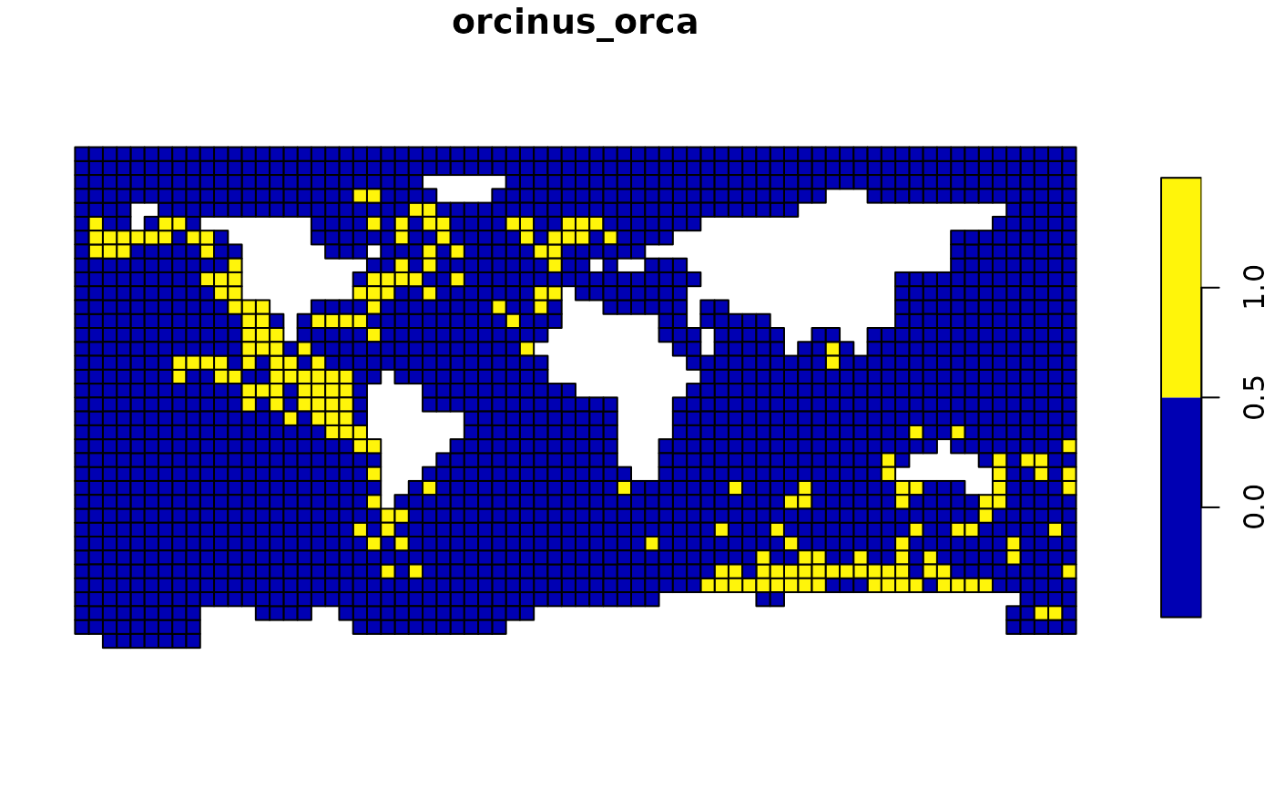
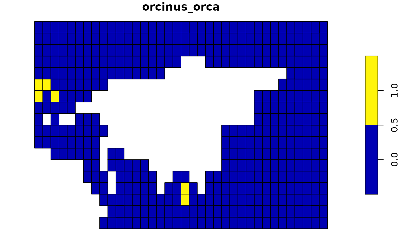
The example below shows how you can filter a specific quadrant from the global killer whale data set using a wildcard notation.

library(dplyr, warn.conflicts = FALSE)
library(sf, warn.conflicts = FALSE)
#> Linking to GEOS 3.10.2, GDAL 3.4.1, PROJ 8.2.1; sf_use_s2() is TRUE

orca_sf <-
  orca |>
  as_csquares(csquares = "csquares") |>
  st_as_sf()

plot(orca_sf["orcinus_orca"])


## Note that the first number in the csquares code (1)
## represents the North East quadrant
## The remainder of the code consists of wildcards.
plot(
  orca_sf |>
    filter(
      in_csquares(csquares, "1***:*")
    ) |>
    drop_csquares() |>
    select("orcinus_orca")
)

Mode

Consider the following csquares object:

csq_example <- as_csquares(c("1000:100|1000:111|1000:206|1000:207", "1000:122"))

It is a vector of two elements, the first containing 4 squares, the second 1 square. Let’s say we want to check if "1000:1**" matches with any of the elements in the vector.

in_csquares(csq_example, "1000:1**")
#> [1] TRUE TRUE

Which is TRUE for both elements in the vector. This makes sense as both elements indeed contain csquares codes that match with "1000:1**". However, the first element also contains elements that don’t match. The reason that the example still returns TRUE in both cases is because the mode is set to "any". Meaning that it will return TRUE if any of the codes in an element matches. You should set the mode to "all" if you only want a positive match when all codes in an element match:

in_csquares(csq_example, "1000:1**", mode = "all")
#> [1] FALSE  TRUE

Strict

Now, let’s compare the same csquares object with "1000:*" which has a lower resolution than the squares in the object:

in_csquares(csq_example, "1000:*")
#> [1] TRUE TRUE

Again, it matches with all elements in the vector, even though the resolution is different. This is because in_csquares() isn’t very strict by default. Meaning that it will also match with any ‘child’ square with a higher resolution. If you want a strict match where the resolution also matches use strict = TRUE:

in_csquares(csq_example, "1000:*", strict = TRUE)
#> [1] FALSE FALSE