Using stars_proxy Objects

Using stars_proxy objects in combination with the CopernicusMarine package introduces opportunities to efficiently work with Data from Copernicus Marine services on the fly.

The great thing about these proxy objects is that they will not read any data unless it is needed. So, you can connect to a dataset from the Copernicus server without having to read raster data. Instead it will only collect meta data about the raster’s dimensions and bands (attributes). The actual raster data is only downloaded when you need it.

Setting Up a Proxy Object

You can either set up a proxy object by calling cms_native_proxy() or cms_zarr_prox(). The first uses the ‘native’ service. In this case the data is already structured in chunked files and the added value of proxy objects is not that obvious. Therefore, in this vignette, we will focus on objects created with cms_zarr_proxy(). It will connect with an entire layer in a product.

library(CopernicusMarine)
library(stars, quietly = TRUE)
#> Linking to GEOS 3.12.1, GDAL 3.8.4, PROJ 9.4.0; sf_use_s2() is TRUE

my_proxy_gc <- cms_zarr_proxy(
  product       = "GLOBAL_ANALYSISFORECAST_PHY_001_024",
  layer         = "cmems_mod_glo_phy-thetao_anfc_0.083deg_P1D-m",
  asset         = "geoChunked")

my_proxy_tc <- cms_zarr_proxy(
  product       = "GLOBAL_ANALYSISFORECAST_PHY_001_024",
  layer         = "cmems_mod_glo_phy-thetao_anfc_0.083deg_P1D-m",
  asset         = "timeChunked")

print(my_proxy_tc)
#> stars_proxy object with 1 attribute in 1 file(s):
#> $thetao
#> [1] "[...]/timeChunked.zarr"
#> 
#> dimension(s):
#>           from   to     offset  delta  refsys
#> longitude    1 4320         NA     NA      NA
#> latitude     1 2041         NA     NA      NA
#> elevation    1   50         NA     NA udunits
#> time         1 1367 2022-06-01 1 days    Date
#>                                                            values x/y
#> longitude            [-180.0417,-179.9583),...,[179.875,179.9584) [x]
#> latitude            [-80.04167,-79.95833),...,[89.95834,90.04166) [y]
#> elevation [-5727.917,-5274.784) [m],...,[-0.494025,0.5533251) [m]    
#> time                                                         NULL

Selecting an Asset Type

The only downside from working with proxy objects is that you need to know which asset type you wish to use. When subsetting data with cms_download_subset() this selection is automated based on your selection criteria. But when working with a proxy object, you may not know which slices you wish to select in advance.

In general, if you wish to work with long time-series in a small geographical area, it’s most efficient to work with "geoChunked" data. Whereas, if you want to work with a short time period, but on a large geographical scale, it is better to use "timeChunked" data.

Slicing a Proxy Object

As you can see from the proxy object printed above, it has dimension that stretch pretty far. It has daily data for nearly four years, in 50 depth layers with global coverage. If you would try to read this raster data, it will almost certainly fail as it would require thousands of Gb of memory which is simply not available on most devices.

Fortunately, the proxy object can easily be sliced, by selecting index values with the bracket operator ([). The first index represents the band (attribute), and we skip it, next are the x and y coordinate, followed by the elevation. The last dimension is time, were we select the first four hundred records.

time_slice <- my_proxy_gc[,2000, 1000, 48, 1:400]
show(time_slice)
#> stars_proxy object with 1 attribute in 1 file(s):
#> $thetao
#> [1] "[...]/geoChunked.zarr"
#> 
#> dimension(s):
#>           from   to     offset  delta  refsys              values x/y
#> longitude 2000 2000         NA     NA      NA     [-13.46,-13.37) [x]
#> latitude  1000 1000         NA     NA      NA       [3.208,3.292) [y]
#> elevation   48   48         NA     NA udunits [-2.646,-1.541) [m]    
#> time         1  400 2022-06-01 1 days    Date                NULL

As you can notice, this slicing is super fast. This is because no actual data is transfered yet. It isn’t until st_as_stars() is called when the data is downloaded. Since in this particular case we have only selected a single raster cell, it makes sense to cast the object to a data.frame. We can then plot the time series.

time_slice <- st_as_stars(time_slice)
plot(st_get_dimension_values(time_slice, "time"), time_slice$thetao,
     xlab = "date", ylab = "temperature", type = "l")

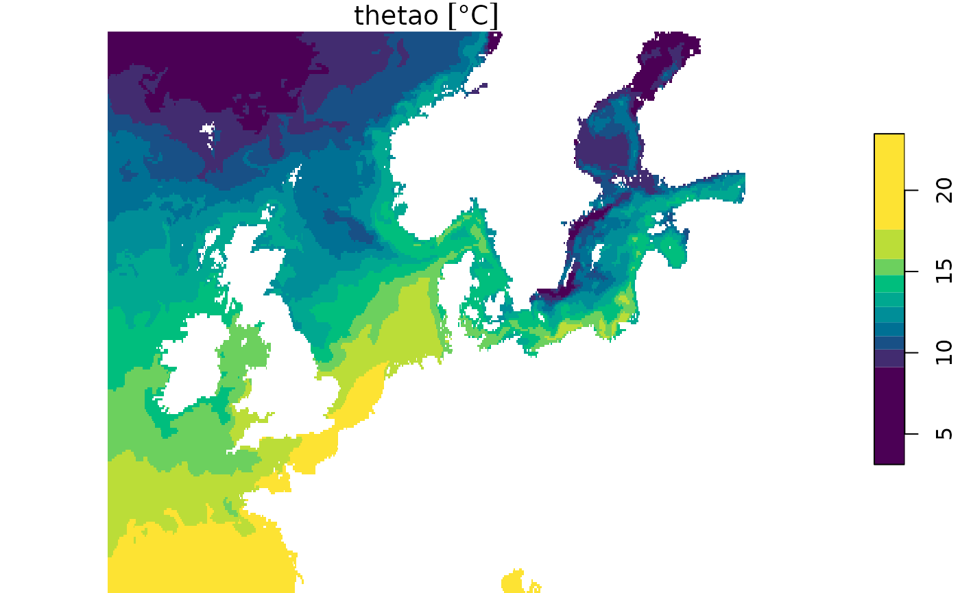
We can also select a specific area, for which we will use the time chunked proxy.

geo_slice <- my_proxy_tc[,2000:2500, 1500:1750, 50, 500]
plot(geo_slice, col = hcl.colors(10))