Image dithering

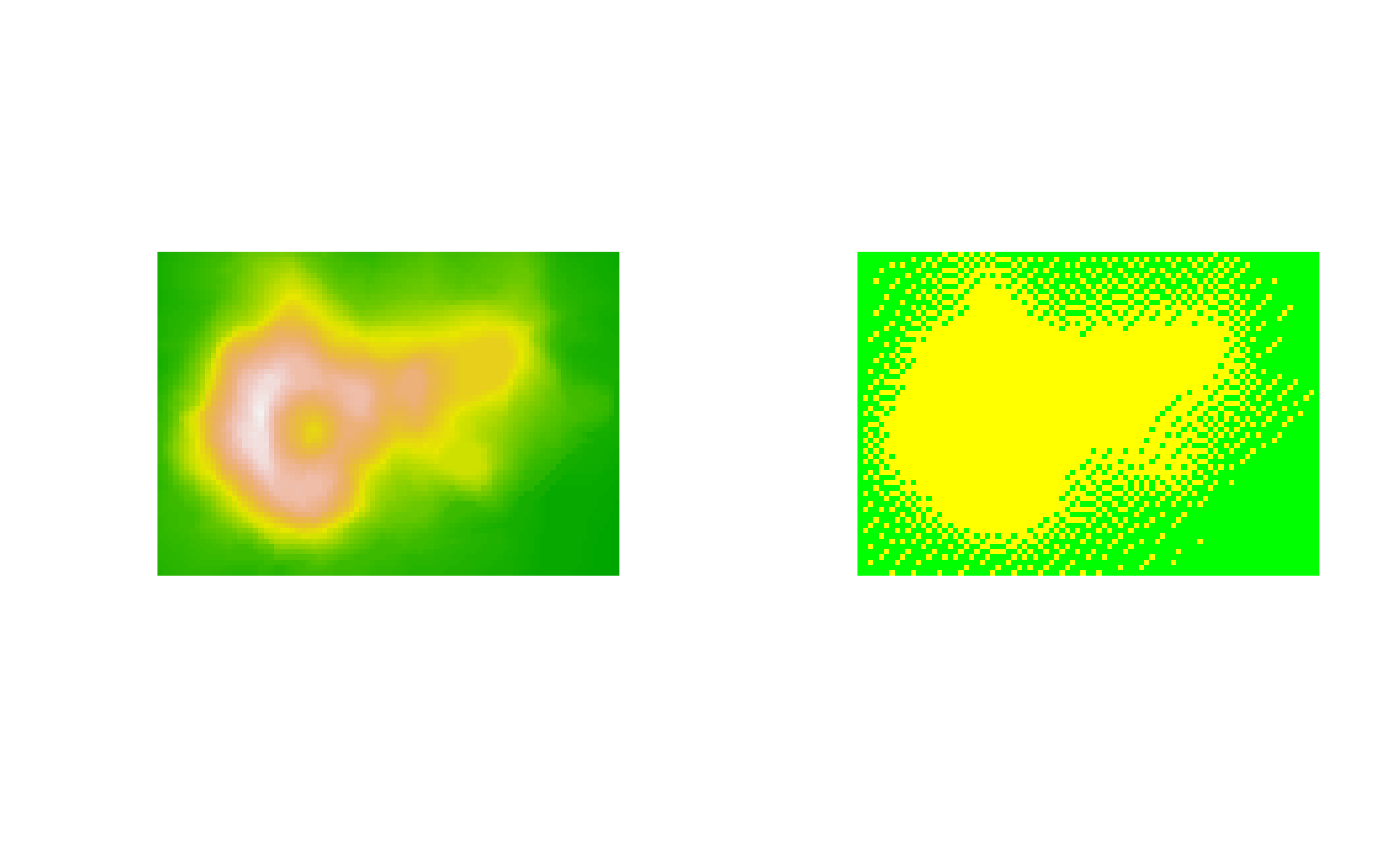
Dither is an intentional form of noise applied to an image to avoid colour banding when reducing the amount of colours in that image. This function applies dithering to a grDevices raster image.

Usage

dither(x, method, ...)

# S3 method for raster
dither(
  x,
  method = c("none", "floyd-steinberg", "JJN", "stucki", "atkinson", "burkse", "sierra",
    "two-row-sierra", "sierra-lite"),
  palette,
  mode = c("none", "HAM6", "HAM8"),
  ...
)

# S3 method for matrix
dither(
  x,
  method = c("none", "floyd-steinberg", "JJN", "stucki", "atkinson", "burkse", "sierra",
    "two-row-sierra", "sierra-lite"),
  palette,
  mode = c("none", "HAM6", "HAM8"),
  ...
)

Arguments

x: Original image data that needs to be dithered. Should be a raster object (grDevices::as.raster()), or a matrix of character string representing colours.
method: A character string indicating which dithering method should be applied. See usage section for all possible options (Note that the "JJN" is the Jarvis, Judice, and Ninke algorithm). Default is "none", meaning that no dithering is applied.
...: Currently ignored.
palette: A palette to which the image should be dithered. It should be a vector of character strings representing colours.
mode: A character string indicating whether a special Amiga display mode should be used when dithering. By default ‘none’ is used (no special mode). In addition, ‘HAM6’ and ‘HAM8’ are supported. See rasterToBitmap() for more details.

Value

Returns a matrix with the same dimensions as x containing numeric index values. The corresponding palette is returned as attribute, as well as the index value for the fully transparent colour in the palette.

Details

The approaches implemented here all use error diffusion to achieve dithering. Each pixel is scanned (from top to bottom, from left to right), where the actual colour is sampled and compared with the closest matching colour in the palette. The error (the differences between the actual and used colour) is distributed over the surrounding pixels. The only difference between the methods implemented here is the way the error is distributed. The algorithm itself is identical. For more details consult the listed references.

Which method results in the best quality image will depend on the original image and the palette colours used for dithering, but is also a matter of taste. Note that the dithering algorithm is relatively slow and is provided in this package for your convenience. As it is not in the main scope of this package you should use dedicated software for faster/better results.

References

R.W. Floyd, L. Steinberg, An adaptive algorithm for spatial grey scale. Proceedings of the Society of Information Display 17, 75-77 (1976).

J. F. Jarvis, C. N. Judice, and W. H. Ninke, A survey of techniques for the display of continuous tone pictures on bilevel displays. Computer Graphics and Image Processing, 5:1:13-40 (1976).

https://en.wikipedia.org/wiki/Floyd-Steinberg_dithering

https://tannerhelland.com/4660/dithering-eleven-algorithms-source-code/

Author

Pepijn de Vries

Examples

if (FALSE) {
## first: Let's make a raster out of the 'volcano' data, which we can use in the example:
volcano.raster <- as.raster(t(matrix(terrain.colors(1 + diff(range(volcano)))[volcano -
  min(volcano) + 1], nrow(volcano))))

## let's dither the image, using a predefined two colour palette:
volcano.dither <- dither(volcano.raster,
                         method = "floyd-steinberg",
                         palette = c("yellow", "green"))

## Convert the indices back into a raster object, such that we can plot it:
volcano.dither <- as.raster(apply(volcano.dither, 2, function(x) c("yellow", "green")[x]))
par(mfcol = c(1, 2))
plot(volcano.raster, interpolate = F)
plot(volcano.dither, interpolate = F)

## results will get better when a better matching colour palette is used.
## for that purpose use the function 'index.colours'.
}