Use a lossy delta-Fibonacci (de)compression to continuous 8-bit signals. This algorithm was used to compress 8-bit audio wave data on the Amiga.
Details
This form of compression is lossy, meaning that information and quality will get lost. 8-bit audio is normally stored as an 8-bit signed value representing the amplitude at specific time intervals. The delta-Fibonacci compression instead stores the difference between two time intervals (delta) as a 4-bit index. This index in turn represents a value from the Fibonacci series (hence the algorithm name). The compression stores small delta values accurately, but large delta values less accurately. As each sample is stored as a 4-bit value instead of an 8-bit value, the amount of data is reduced with almost 50\
The algorithm was first described by Steve Hayes and was used in 8SVX audio stored in the Interchange File Format (IFF). The quality loss is considerable (especially when the audio contained many large deltas) and was even in the time it was developed (1985) not used much. The function is provided here for the sake of completeness. The implementation here only compresses 8-bit data, as for 16-bit data the quality loss will be more considerable.
References
https://en.wikipedia.org/wiki/Delta_encoding
http://amigadev.elowar.com/read/ADCD_2.1/Devices_Manual_guide/node02D6.html
Examples
## Let's get an audio wave from the ProTrackR package, which we
## can use in this example:
buzz     <- ProTrackR::PTSample(ProTrackR::mod.intro, 1)

## Let's convert it into raw data, such that we can compress it:
buzz.raw <- as.integer(ProTrackR::waveform(buzz) - 128) |>
  bitwAnd(0xFF) |>
  as.raw()

## Let's compress it:
buzz.compress <- deltaFibonacciCompress(buzz.raw)

## Look the new data uses less memory:
length(buzz.compress)/length(buzz.raw)
#> [1] 0.5019231

## The compression was lossy, which we can examine by decompressing the
## sample again:
buzz.decompress <- deltaFibonacciDecompress(buzz.compress)

## And turn the raw data into numeric data:
buzz.decompress <-
  ifelse(buzz.decompress > 0x7f, as.integer(buzz.decompress) - 256L,
         as.integer(buzz.decompress))

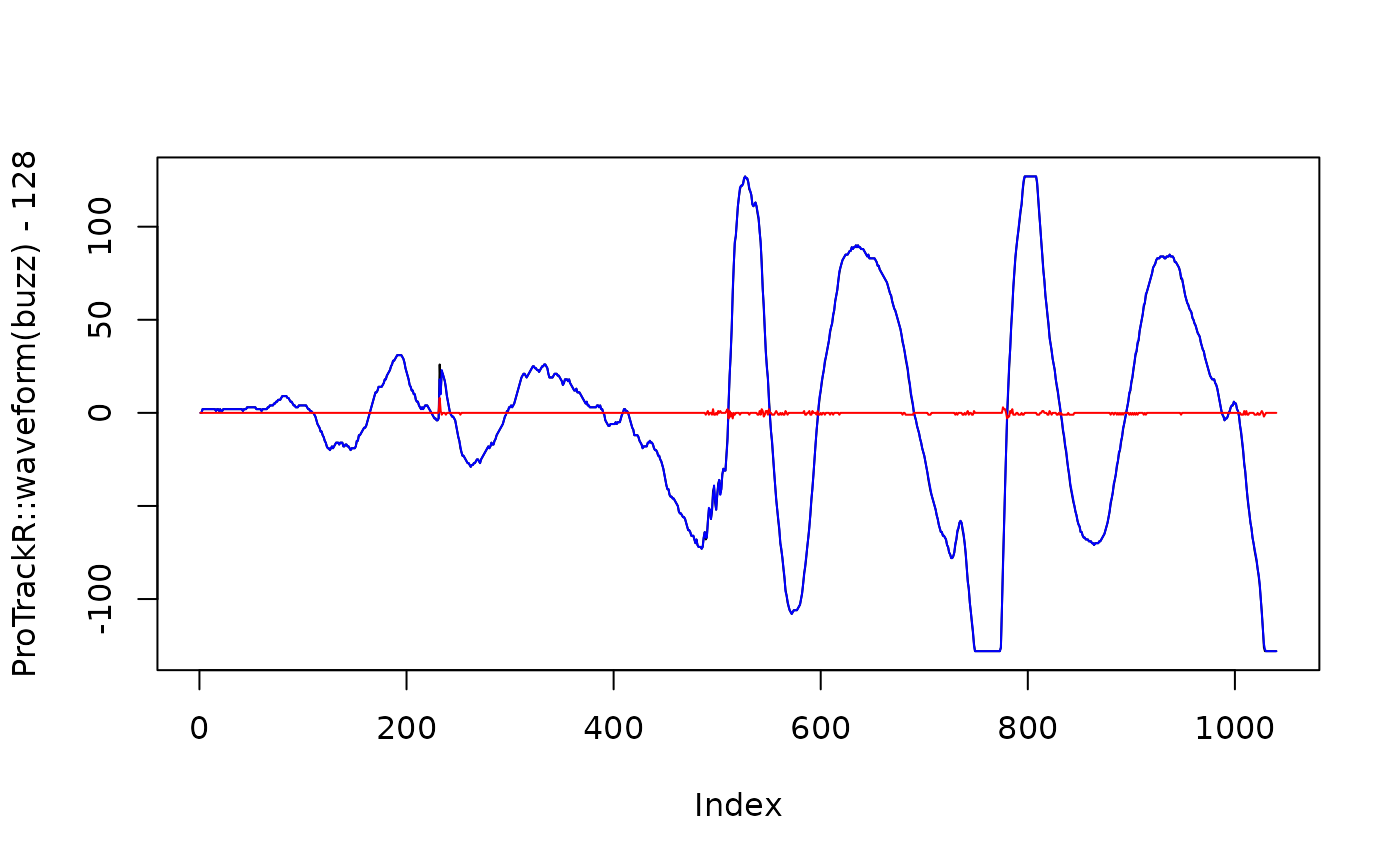
## Plot the original wave in black, the decompressed wave in blue
## and the error in red (difference between the original and decompressed
## wave). The error is actually very small here.
plot(ProTrackR::waveform(buzz) - 128, type = "l")
lines(buzz.decompress, col = "blue")
buzz.error <- ProTrackR::waveform(buzz) - 128 - buzz.decompress
lines(buzz.error, col = "red")


## this can also be visualised by plotting the orignal wave data against
## the decompressed data (and observe a very good correlation):
plot(ProTrackR::waveform(buzz) - 128, buzz.decompress)


## Let's do the same with a sample of a snare drum, which has larger
## delta values:
snare.drum <- ProTrackR::PTSample(ProTrackR::mod.intro, 2)

## Let's convert it into raw data, such that we can compress it:
snare.raw <- as.integer(ProTrackR::waveform(snare.drum) - 128L) |>
  bitwAnd(0xFF) |>
  as.raw()

## Let's compress it:
snare.compress <- deltaFibonacciCompress(snare.raw)

## Decompress the sample:
snare.decompress <- deltaFibonacciDecompress(snare.compress)

## And turn the raw data into numeric data:
snare.decompress <-
  ifelse(snare.decompress > 0x7f, as.integer(snare.decompress) - 256L,
         as.integer(snare.decompress))

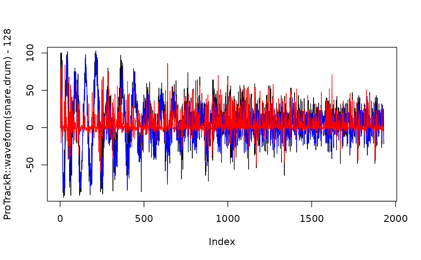
## Now if we make the same comparison as before, we note that the
## error in the decompressed wave is much larger than in the previous
## case (red line):
plot(ProTrackR::waveform(snare.drum) - 128, type = "l")
lines(snare.decompress, col = "blue")
snare.error <- ProTrackR::waveform(snare.drum) - 128 - snare.decompress
lines(snare.error, col = "red")


## this can also be visualised by plotting the orignal wave data against
## the decompressed data (and observe a nice but not perfect correlation):
plot(ProTrackR::waveform(snare.drum) - 128, snare.decompress)
