Calculate correction for angle in the plot coordinate system
Source:R/angle_correction.r
angle_correction.Rd
The angle of a vector may be distorted when your plot uses a different
coordinate system than the one for which the angle is specified. If data
is a simple feature object (sf), the angle will be corrected
for the displayed coordinate reference system (crs). When
the crs is missing, an aspect ratio of 1 is assumed. For any other data,
the angle is corrected for the aspect ratio in the plot.
Arguments
- data
fortified data used in a
geom_fields()
. Should at least containnumeric
columnsx
,y
andangle
.- panel_params
panel parameters as returned by GeomFields$setup_params()
- coord
A coord object.
Value
A data.frame
with an additional angle_correction
column. The corrected angle is given
by angle_correction + angle
.
Details
This function is used by default by geom_fields()
. For more details on
why this correction is required and how to customize corrections please see
vignette("angle_correction")
.
Examples
## Create a data.frame with some xy-coordinates and all angles pointing North (0 degrees)
d <-
data.frame(
x = seq(1, 2, 0.1),
y = seq(50, 51, 0.1),
angle = 0
) |>
sf::st_as_sf(coords = c("x", "y"), crs = 4326, remove = FALSE)
## Create a mockup of ggplot params. Normally this is handled automatically by ggplot2
params_mockup <-
c(
ggplot2::ggplot() + geom_fields(),
list(
x_range = range(d$x),
y_range = range(d$y),
crs = sf::st_crs(4326),
default_crs = 4326
)
)
## When plotting as lon-lat, the angle correction will be zero
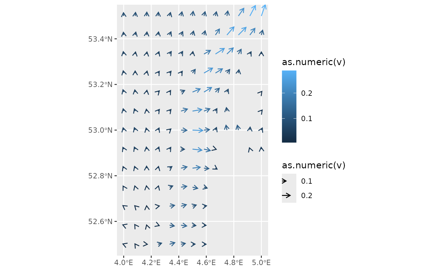
angle_correction(d, params_mockup, ggplot2::coord_sf(default_crs = 4326))
#> Angle correction between 0.00 and 0.00 radials
#> Simple feature collection with 11 features and 4 fields
#> Geometry type: POINT
#> Dimension: XY
#> Bounding box: xmin: 1 ymin: 50 xmax: 2 ymax: 51
#> Geodetic CRS: WGS 84
#> First 10 features:
#> x y angle geometry angle_correction
#> 1 1.0 50.0 0 POINT (1 50) 0
#> 2 1.1 50.1 0 POINT (1.1 50.1) 0
#> 3 1.2 50.2 0 POINT (1.2 50.2) 0
#> 4 1.3 50.3 0 POINT (1.3 50.3) 0
#> 5 1.4 50.4 0 POINT (1.4 50.4) 0
#> 6 1.5 50.5 0 POINT (1.5 50.5) 0
#> 7 1.6 50.6 0 POINT (1.6 50.6) 0
#> 8 1.7 50.7 0 POINT (1.7 50.7) 0
#> 9 1.8 50.8 0 POINT (1.8 50.8) 0
#> 10 1.9 50.9 0 POINT (1.9 50.9) 0
## Transform to UTM zone 31N in meters
d2 <- d |> sf::st_transform(32631)
## Again get parameter mockup values
params_mockup2 <-
c(
ggplot2::ggplot() + geom_fields(),
list(
x_range = range(sf::st_coordinates(d2)[,1]),
y_range = range(sf::st_coordinates(d2)[,1]),
crs = sf::st_crs(32631),
default_crs = 4326
)
)
## in UTM projection in this area (which is slightly tilted) the correction is
## larger than zero
angle_correction(d2, params_mockup2,
ggplot2::coord_sf(crs = 32631, default_crs = 4326))
#> Angle correction between 0.01 and 0.03 radials
#> Simple feature collection with 11 features and 4 fields
#> Geometry type: POINT
#> Dimension: XY
#> Bounding box: xmin: 356670.9 ymin: 5540547 xmax: 429831.1 ymax: 5650301
#> Projected CRS: WGS 84 / UTM zone 31N
#> First 10 features:
#> x y angle geometry angle_correction
#> 1 1.0 50.0 0 POINT (356670.9 5540547) 0.02674472
#> 2 1.1 50.1 0 POINT (364119.6 5551478) 0.02544421
#> 3 1.2 50.2 0 POINT (371539 5562419) 0.02413979
#> 4 1.3 50.3 0 POINT (378929 5573369) 0.02283147
#> 5 1.4 50.4 0 POINT (386289.6 5584330) 0.02151924
#> 6 1.5 50.5 0 POINT (393620.7 5595300) 0.02020311
#> 7 1.6 50.6 0 POINT (400922.2 5606280) 0.01888310
#> 8 1.7 50.7 0 POINT (408194.1 5617271) 0.01755922
#> 9 1.8 50.8 0 POINT (415436.2 5628271) 0.01623147
#> 10 1.9 50.9 0 POINT (422648.6 5639281) 0.01489986